Imputing electoral Census data for election years

## ── Attaching core tidyverse packages ──────────────────────── tidyverse 2.0.0 ──
## ✔ dplyr     1.1.2     ✔ readr     2.1.4
## ✔ forcats   1.0.0     ✔ stringr   1.5.0
## ✔ ggplot2   3.4.2     ✔ tibble    3.2.1
## ✔ lubridate 1.9.2     ✔ tidyr     1.3.0
## ✔ purrr     1.0.1     
## ── Conflicts ────────────────────────────────────────── tidyverse_conflicts() ──
## ✖ dplyr::filter() masks stats::filter()
## ✖ dplyr::lag()    masks stats::lag()
## ℹ Use the conflicted package (<http://conflicted.r-lib.org/>) to force all conflicts to become errors

Introduction

A Census is conducted every five years by the Australian Bureau of Statistics. In the years 2001 and 2016 both a federal election and Census occur, but in the other election years (2004, 2007, 2010 and 2013) there is no Census to directly match, so Census data from neighbouring years must be used in any modelling. This vignette documents how to impute Census data for the desired election year, which involves interpolating between the neighbouring Censuses.

We impute Census data for the electoral divisions in the 2013 federal election. Maps of 2013 and 2016 electoral divisions are obtained from the Australian Electoral Commission http://www.aec.gov.au/Electorates/gis/gis_datadownload.htm, and the map of divisions in place at the time of the 2011 Census is from the Australian Bureau of Statistics https://datapacks.censusdata.abs.gov.au/datapacks/.

The Australian Electoral Commission shifts the electoral boundaries regularly, so the electoral divisions in place in the 2013 election may not match those in 2016, nor those in 2011. This means that obtaining Census information for a particular electoral division, we are not necessarily able to directly interpolate between the electoral Census profiles in neighbouring Censuses.

To account for these boundary shifts, we use a spatio-temporal algorithm to estimate Census information about each electorate, at the time of the election of interest. Electoral boundaries are superimposed onto each of the neighbouring Censuses, in order to estimate Census characteristics for each of those years. By linearly interpolating between these time points, we get an estimate for the election year of interest.

To illustrate this algorithm, consider the example Melbourne Ports, an electoral division in the 2013 federal election.

Example: Melbourne Ports in the 2013 election

To illustrate the spatio-temporal algorithm, consider the imputation of a socio-demographic variable for the electorate of Melbourne Ports in Victoria (VIC), at the time of the 2013 federal election. The figure below shows this region amongst other VIC electorates.

# Data available in extra-data folder of github repo
load("../extra-data/vic_map.rda")

p1 <- ggplot(data = vic_map) +
  geom_polygon(aes(x = long, y = lat, group = group, fill = Elect_div == "Melbourne Ports"),
    colour = "black", alpha = 0.4
  ) +
  scale_fill_manual(
    name = "Electoral Boundaries",
    values = c("white", "purple"),
    labels = c("Other Electorates", "Melbourne Ports (VIC)")
  ) +
  theme_map() +
  coord_equal(xlim = c(144.88, 145.07), ylim = c(-37.92, -37.78))

p1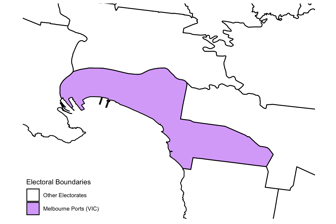

Some of the electoral boundaries in NSW for 2013, with the electoral boundary for Hume, shown in purple.

The Censuses neighbouring the 2013 election are those in 2011 and 2016. From each Census, the most disaggregate data that is publicly available is used - Statistical Area 1. There were approximately 55,000 SA1s in the 2016 Census (meaning approximately 400 people are contained in each SA1). For simplicity, each SA1 is summarised by its centroid. Each SA1 centroid that falls within the 2013 Melbourne Ports boundary is assigned to the Melbourne Ports electorate for 2013.

The centroids are held in the extra-data folder in the eechidna github repo.

load("../extra-data/centroids_sa1_2011.rda")

# Load centroids in this window (pre-prepared)
load("../extra-data/MP_sa1_dots_2011.rda")

p1 + geom_point(aes(x = long_c, y = lat_c, shape = shape), data = MP_sa1_dots_2011 %>% mutate(shape = "1"), colour = "grey25", size = 1.3) + scale_shape_manual(name = "Statistical Area 1", values = 3, labels = "Centroids")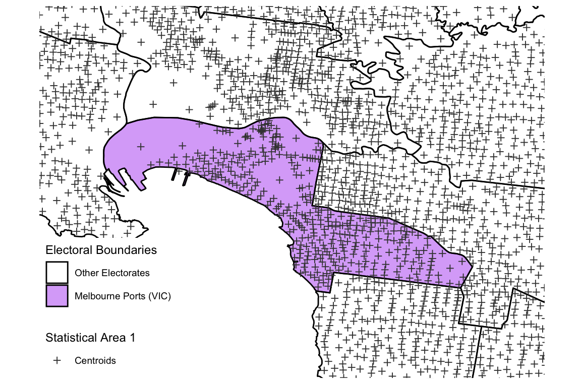

Melbourne Ports boundary and surrounding electorates from 2013, with the SA1 centroids from the 2016 Census shown. Centroids falling within the purple region are assigned to Melbourne Ports.

Formally, let $I_{s,t}$ be an indicator variable, for which $I_{s,t} = 1$ if the centroid of source zone $s$ falls within target zone $t$, and $0$ otherwise. Additionally, let the population of the source zone $s$ be $U_s$ and the population of target zone $t$ be $P_{t}$.

In order to calculate socio-demographic information for each of the electoral boundaries, a weighted average of SA1 characteristics is taken using their populations as weights. Denote a given Census variable for the target zone by $C_t$, and the same Census variable for the source zone as $D_s$. Then, estimate $C_t$ using \[ \hat{C}_t = \frac{\sum_{s=1}^{S}{I_{s,t}*D_s*U_s}}% {\sum_{s=1}^{S}{I_{s,t}*U_s}}, \quad\text{for each $t=1,\dots,T$}. \]

To account for temporal changes, linear interpolation is used between Census years to get the final estimate of a Census variable for the target zone in the election year. Let $y_1$ be the year of the Census preceding an election, let $y_2$ be the year of the election, and $y_3$ be the year of the Census that follows. Add this year subscript to the Census variable estimate $\hat{C}_t$, resulting in $\hat{C}_{t,y}$. Linear interpolating between these Census years results an imputed value for the election year, given by \[ \hat{C}_{t,y_2} = \frac{y_3-y_2}{y_3-y_1} \hat{C}_{t,y_1} + \frac{y_2-y_1}{y_3-y_1} \hat{C}_{t,y_3}. \]

Continuing with the example of Melbourne Ports in the 2013 election, the estimate for a given Census variable in 2016, $\hat{C}_{\text{MelbPorts}, 2016}$ would be obtained by computing the weighted average of this variable amongst the SA1s within the purple region shown in Figure @ref(fig:melb_ports13). This would be repeated with the 2011 Census SA1s to obtain $\hat{C}_{\text{MelbPorts}, 2011}$, from which the final estimate is given by \[ \hat{C}_{\text{MelbPorts},2013} = \frac{3}{5} \hat{C}_{\text{MelbPorts},2011} + \frac{2}{5} \hat{C}_{\text{MelbPorts},2016}. \] This is done for each of the socio-demographic variables, and is repeated for each of the 149 remaining electoral boundaries corresponding with 2013 electorates.

Imputing all electorates in the 2013 election

aec_sF is the shapefile containing the polygons associated with electoral boundaries for which Census information is to be imputed, and abs_sF contains SA1 polygons from the Census.

First load the shapefile containing the electoral boundaries from the 2013 federal election, sF_13.

sF_13 <- load_shapefile("path-to-your-shapefiles/national-midmif-16122011/COM20111216_ELB.MIF")

Then extract the centroids from the 2011 Census SA1 polygons from the object sF_11_sa1. Here we use the function extract_centroids. Note that sF_11_sa1 is too large an object for demonstration but it can be downloaded from https://datapacks.censusdata.abs.gov.au/datapacks/.

centroids_sa1_2011 <- extract_centroids(sF11_sa1)

Now use the function allocate_electorate to allocate each SA1 to the electoral boundary in which it sits.

mapping_c11_e13 <- allocate_electorate(centroids_ls = centroids_sa1_2011, electorates_sf = sF_13, census_year = "2011", election_year = "2013")

Next the weighted_avg_census_sa1 function applies a weighted average of SA1 characteristics for each electorate using the SA1 populations as weights. This uses abs2011_cd which is the equivalent of abs2011 in eechidna1, but with each row corresponding with an SA1. Again, this is too large to include in the repo.

census_aec13_11 <- weighted_avg_census_sa1(mapping_df = mapping_c11_e13, abs_df = abs2011_cd)

We repeat this for the 2016 Census.

centroids_sa1_2016 <- extract_centroids(sF16_sa1)
mapping_c16_e13 <- allocate_electorate(centroids_ls = centroids_sa1_2016, electorates_sf = sF_13, census_year = "2016", election_year = "2013")
census_aec13_16 <- weighted_avg_census_sa1(mapping_df = mapping_c16_e13, abs_df = abs2016_cd)

Now we can linearly interpolate between 2011 and 2016 to arrive at our final estimate of Census data for the electorates in place at the 2013 federal election. This involves using inverse distance weighting (power of 1).

# Linearly interpolate using inverse distance weighting (power of 1)
abs2013 <- (2/5)*(select(census_aec13_16, -DivisionNm)) + (3/5)*(select(census_aec13_11, -DivisionNm))

# Maintain division names
abs2013$DivisionNm <- census_aec13_16$DivisionNm

abs2013 %>% select(DivisionNm, Age00_04, Age05_14, Age15_19, BachelorAbv, MedianPersonalIncome, Owned, NoReligion) %>%
  head() %>% 
  kable

DivisionNm	Age00_04	Age05_14	Age15_19	BachelorAbv	MedianPersonalIncome	Owned	NoReligion
ADELAIDE	5.233431	9.525292	5.798392	32.026265	479.2099	28.92356	30.89500
ASTON	5.857371	12.317517	7.088707	20.278193	458.3521	34.28622	27.50937
BALLARAT	6.502042	12.982534	6.914297	16.500943	406.2691	34.17926	31.20523
BANKS	6.056353	11.479071	6.174769	24.902730	421.4060	34.85625	22.54929
BARKER	5.949816	12.904095	6.215134	8.145889	386.6909	36.01356	30.27061
BARTON	6.330059	10.807894	5.271060	23.877154	435.3009	36.15573	16.12376

Summary

We have demonstrated how to use the functions needed to impute Census information for 2004, 2007, 2010 and 2013 elections. For future elections, the same functions can be used, and rather than interpolating over time, simply use the previous Census, until another Census is made available (as we have done with 2019).

Jeremy Forbes

2023-04-26

Introduction

Example: Melbourne Ports in the 2013 election

Imputing all electorates in the 2013 election

Summary