Getting Oz Electorate shapefiles into shape

Heike Hofmann, Di Cook and Jeremy Forbes

2023-04-26

This vignette details the procedure used to obtain the maps of electoral boundaries for each of the Australian federal elections and Censuses.

The Australian Electorate Commission publishes the boundaries of the electorates on their website at http://www.aec.gov.au/Electorates/gis/gis_datadownload.htm (2010-2016). Electoral boundaries for 2001 are sourced from the Australian Government at https://data.gov.au/. The 2004 and 2007 electoral boundaries are available from the Australian Bureau of Statistics http://www.abs.gov.au/AUSSTATS/abs@.nsf/DetailsPage/2923.0.30.0012006?OpenDocument.

Once the files (preferably the national files) are downloaded, unzip the file (it will build a folder with a set of files). We want to read the shapes contained in the shp, TAB, or MIF file into R. The rgdal library can be used to do this.

The function get_electorate_shapes in this package extracts a list from the shapefile, consisting of a dataframe containing coordinates of each polygon and a dataframe with data associated with each polygon (electorate). These can be used directly with ggplot graphics. Alternatively, the load_shapefile function (also from eechidna) imports the shapefile as a SpatialPolygonsDataFrame.

library(eechidna)
# shapeFile contains the path to the shp file:
shapeFile <- "/PATH-ON-YOUR-COMPUTER/2021_ELB_region.shp"
map_and_data <- get_electorate_shapes(shapeFile)

nat_map <- map_and_data$map
nat_data <- map_and_data$data

Here we have a map of the Australian electorates colored by their size as given in the data (variable area_sqkm):

library(ggplot2)
library(ggthemes)
library(ggmap)

ggplot(aes(map_id=id), data=nat_data) +
  geom_map(aes(fill=area_sqkm), map=nat_map) +
  expand_limits(x=nat_map$long, y=nat_map$lat) + 
  theme_map() + coord_equal()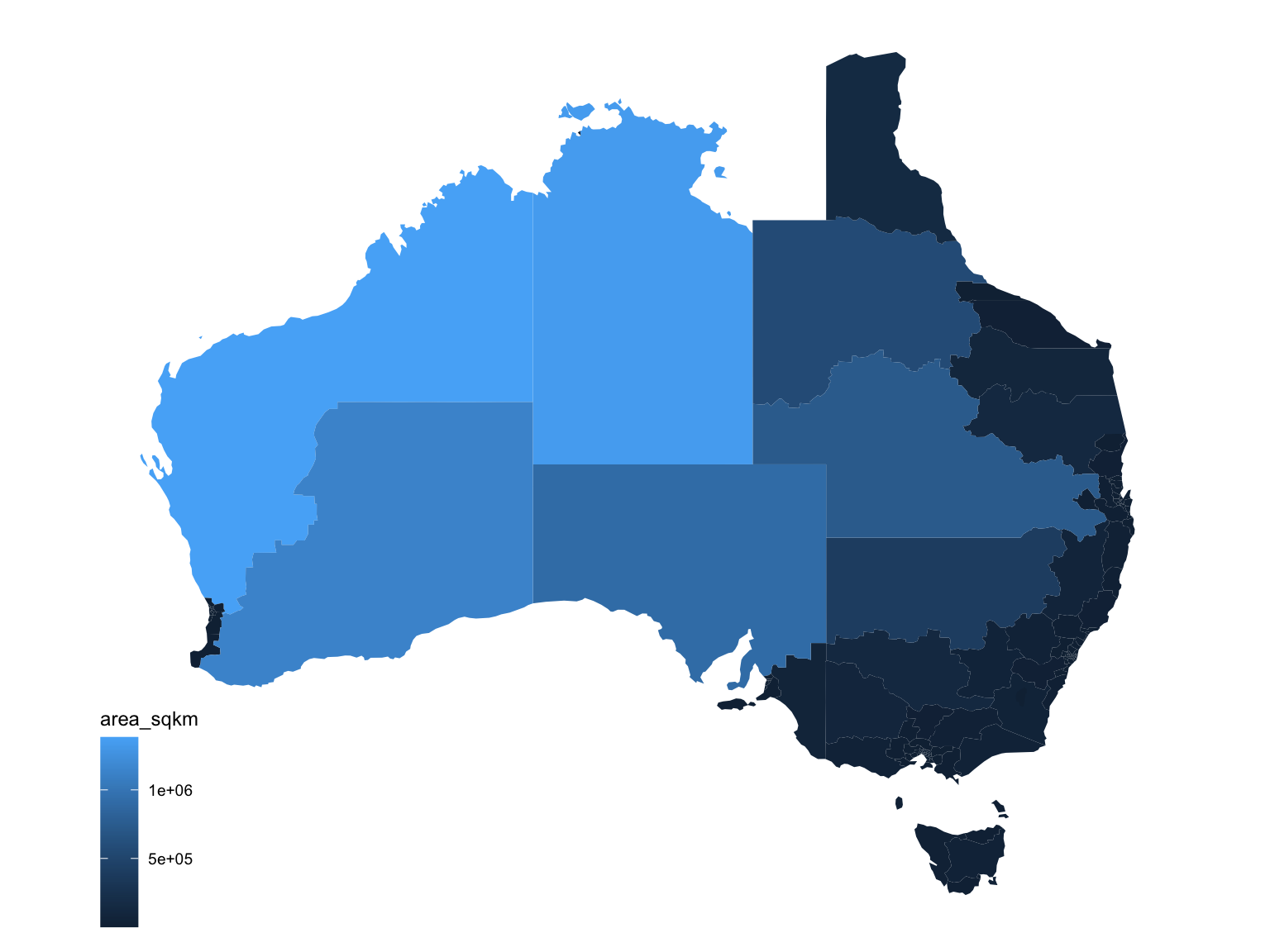

The get_electorate_shapes function was re-written Australian electoral boundaries for 2022, but may need some tweaking for future electoral maps. (Code for previous years can be found in release v1.4.1.) Each step of this function is detailed below, with the running example of the Australian electoral boundaries for 2022.

Steps

For the 2022 election, the national electorate boundaries are given in ESRI shp format.

sF is a spatial data frame containing all of the polygons. First, for convenience, lets change all variable names in the associated data set to lower case.

names(sF) <- tolower(names(sF))

We now use rmapshaper to thin the polygons and ensure that there are no holes while preserving the geography:

library(rmapshaper)

sF_polys <- rmapshaper::ms_simplify(sF, keep = 0.001)

keep is the numerical value indicating proportion of vertices to keep in the map, reducing the number of points. Doing this helps reduce the overall size of the map considerably, making it faster to plot. For data analysis, you don’t need detailed maps.

Extracting the electorate information

A spatial polygons data frame consists of both a data set with information on each of the entities (in this case, electorates), and a set of polygons for each electorate (sometimes multiple polygons are needed, e.g. if the electorate has islands). We want to extract both of these parts.

nat_data <- st_set_geometry(sF, NULL)
head(nat_data)

The row names of the data file are identifiers corresponding to the polygons - we want to make them a separate variable:

nat_data$id <- row.names(nat_data)

In the currently published version of the 2022 electorate boundaries, the data data frame has variable elect_div of the electorates’ names, but not state information. We add this with:

  if (!("state" %in% names(nat_data))) {
    states <- states22
    states$elect_div <- toupper(states$elect_div)
    nat_data <- nat_data %>%
      left_join(states) %>%
      select(id, elect_div, state, numccds, area_sqkm, long_c, lat_c)
  }

giving the column state, which is an abbreviation of the state name. It might be convenient to merge this information (or at least the state abbreviation) into the polygons (see below).

We are almost ready to export this data into a file, but we still want include geographic centers in the data (see also below).

Extracting the polygon information

The sptable function in the spbabel package extracts the polygons into a data frame.

  nat_map <- spbabel::sptable(sF_polys)

We need to make sure that group and piece are kept as factor variables - if they are allowed to be converted to numeric values, it messes things up, because as factor levels 9 and 9.0 are distinct, whereas they are not when interpreted as numbers …

nat_map$group <- paste("g",nat_map$piece, sep=".")

It is useful to have the electorate name and state attached to the map.

nms <- nat_data %>% select(id, elect_div, state)
nat_map$id <- as.character(nat_map$id)
nat_map <- dplyr::left_join(nat_map, nms, by="id")

The map data is ready to be exported to a file:

head(nat_map)

Getting centroids

Getting centroids or any other information from a polygon is fairly simple, once you have worked your way through the polygon structure. The sf package makes this easier to do now. We will wrap this into a little function called centroid to help us with that:

library(purrr)
centroid <- function(i, polys) {
  ctr <- st_centroid(st_geometry(sF)[[i]])
  data.frame(long_c=ctr[1], lat_c=ctr[2])
}

centroids <-  purrr::map_df(1:nrow(sF), centroid, polys=sf)

head(centroids)

The centroids come in the same order as the data (luckily) and we just extend the data set (dropping the geometry) for the electorates by this information, and finally export:

nat_data <- st_set_geometry(sF, NULL)
nat_data <- data.frame(nat_data, centroids)

readr::write_csv(nat_data, "national-data-2022.csv")

Finally, just to check the data, after running get_electorate_shapes(), a map of the Australian electorates colored by their size as given in the data (variable area_sqkm):

ggplot(aes(map_id=id), data=nat_data) +
  geom_map(aes(fill=area_sqkm), map=nat_map) +
  expand_limits(x=nat_map$long, y=nat_map$lat) + 
  theme_map() + coord_equal()