Exploring the Census data: A case study of 2016

Introduction

The eechidna (Exploring Election and Census Highly Informative Data Nationally for Australia) R package makes it easy to look at the Census (and election) data from the 2001, 2006, 2011 and 2016 Australian Censuses.

This vignette documents how to access the Census data, using the example of 2016, and shows a few typical methods that can be used to explore the data.

2016 Census data

The data is loaded as abs2016 when you load eechidna.

library(eechidna)

data(abs2016)

Here we see that we have 150 observations and 86 variables.

Each observation is data pertaining to a particular federal electorate as described by http://www.aec.gov.au/profiles/.

Each variable is described here:

Variable	Details
UniqueID	Commonwealth Electoral District identifier
DivisionNm	Name of electorate
State	State containing electorate
Population	Total population of electorate
Area	Area of electorate division in square kilometres
Age00_04	Percentage of people aged 0-4.
Age05_14	Percentage of people aged 5-9.
Age15_19	Percentage of people aged 15-19.
Age20_24	Percentage of people aged 20-24.
Age25_34	Percentage of people aged 25-34.
Age35_44	Percentage of people aged 35-44.
Age45_54	Percentage of people aged 45-54.
Age55_64	Percentage of people aged 55-64.
Age65_74	Percentage of people aged 65-74.
Age75_84	Percentage of people aged 75-84.
Age85plus	Percentage of people aged 85 or higher.
Anglican	Percentage of people affiliated with the Anglican denomimation
AusCitizen	Percentage of people who are Australian Citizens
AverageHouseholdSize	Average number of people in a household
BachelorAbv	Percentage of people who have completed a Bachelor degree or above
Born_Asia	Percentage of people born in Asia
Born_MidEast	Percentage of people born in the Middle East
Born_SE_Europe	Percentage of people born in South Eastern Europe
Born_UK	Percentage of people born in the United Kingdom
BornElsewhere	Percentage of people born in a different region outside of Australia
BornOverseas_NS	Percentage of people who did not answer the question relating to birthplace
Buddhism	Percentage of people affiliated with the Buddhist religion
Catholic	Percentage of people affiliated with the Catholic denomimation
Christianity	Percentage of people affiliated with the Christian religion (of all denominations)
Couple_NoChild_House	Percentage of households made up of a couple with no children
Couple_WChild_House	Percentage of households made up of a couple with children
CurrentlyStudying	Percentage of people who are currently studying
DeFacto	Percentage of people who are in a de facto marriage
DiffAddress	Percentage of people who live at a different address to what they did 5 years ago
DipCert	Percentage of people who have completed a diploma or certificate (not including graduate diploma)
Distributive	Percentage of employed persons who work in wholesale trade, retail trade, transport, post or warehousing related industries
EmuneratedElsewhere	Percentage of people who receive emuneration outside of Australia, out of the total population plus overseas visitors
EnglishOnly	Percentage of people who speak only English
Extractive	Percentage of employed persons who work in extractive industries (includes mining, gas, water, agriculture, waste, electricity)
FamilyIncome_NS	Percentage of people who did not answer the question relating to family income
FamilyRatio	Average number of people per family
Finance	Percentage of employed persons who work in finance or insurance related industries
HighSchool	Percentage of people who have completed high school
HighSchool_NS	Rate of nonresponse for questions relating to high school completion
HouseholdIncome_NS	Percentage of people who did not answer the question relating to houshold income
Indigenous	Percentage of people who are Indigenous
InternetAccess	Percentage of people with access to the internet
InternetAccess_NS	Rate of nonresponse for questions relating to internal access
InternetUse	Percentage of people who used interent in the last week [2001 only]
InternetUse_NS	Rate of nonresponse for questions relating to internet use [2001 only]
Islam	Percentage of people affiliated with the Islamic religion
Judaism	Percentage of people affiliated with the Jewish religion
Laborer	Percentage of employed persons who work as a laborer
Language_NS	Rate of nonresponse for questions relating to language spoken at home
LFParticipation	Labor force participation rate
ManagerAdminClericalSales	Percentage of employed persons who work in management, administration, clerical duties and sales
Married	Percentage of people who are married
MedianAge	Median age
MedianFamilyIncome	Median weekly family income (in $)
MedianHouseholdIncome	Median weekly household income (in $)
MedianLoanPay	Median mortgage loan repayment amount (of mortgage payments, in $)
MedianPersonalIncome	Median weekly personal income (in $)
MedianRent	Median weekly rental payment amount (of those who rent, in $)
Mortgage	Percentage of dwellings that are on a mortgage
NoReligion	Percentage of people with no religion
OneParent_House	Percentage of households made up of one parent with children
Other_NonChrist	Percentage of people affiliated with a religion other than Christianity, Buddhism, Islam and Judaism
OtherChrist	Percentage of people affiliated with a denomination of the Christian religion other than Anglican or Catholic
OtherLanguageHome	Percentage of people who speak a language other than English at home
Owned	Percentage of dwellings that are owned outright
PersonalIncome_NS	Rate of nonresponse for questions relating to personal income
Professional	Percentage of employed persons who work as a professional
PublicHousing	Percentage of dwellings that are owned by the government, and rented out to tenants
Religion_NS	Rate of nonresponse for questions relating to religion
Rent_NS	Rate of nonresponse for questions relating to rental costs
Renting	Percentage of dwellings that are being rented
SocialServ	Percentage of employed persons who work in education and training, healthcare, wocial work, community, arts and recreation
SP_House	Percentage of households occupied by a single person
Tenure_NS	Rate of nonresponse for questions relating to tenure
Tradesperson	Percentage of employed persons who specialise in a trade
Transformative	Percentage of employed persons who work in construction or manufacturing related industries
Unemployed	Unemployment rate
University_NS	Rate of nonresponse for questions relating to University
Volunteer	Percentage of people who work as a volunteer
Volunteer_NS	Rate of nonresponse for questions relating to working as a volunteer

So let’s just look at some nice and simple plots using ggplot2.

Unemployment

library(ggplot2)
ggplot(data = abs2016,
       aes(x = Unemployed)) + 
  geom_density(fill = "salmon", 
               bw = "SJ",
               colour = NA) + 
  geom_rug(colour = "salmon") +
  theme_minimal() +
  xlim(0, 12)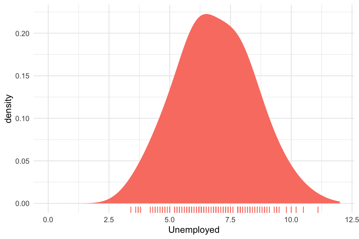

Unemployment by state

ggplot(data = abs2016,
       aes(x = reorder(State, -Unemployed),
           y = Unemployed,
           colour = State)) + 
  geom_boxplot() + 
  labs(x = "State",
       y = "% Unemployment") + 
  theme_minimal() + 
  theme(legend.position = "none")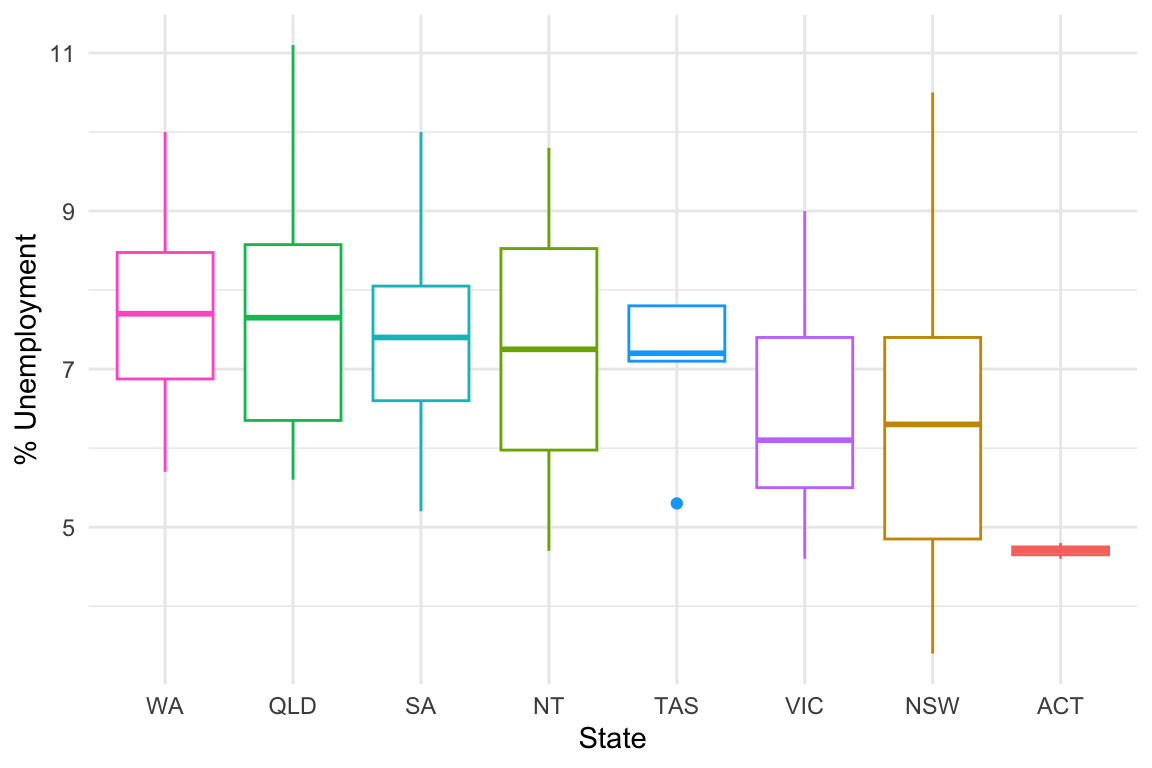

Age

ggplot(data = abs2016,
       aes(x = Age00_04)) +
   geom_density(fill = "steelblue",
               bw = "SJ",
               colour = NA) + 
  xlim(3,11) +
  geom_rug(colour = "steelblue") + 
  theme_minimal() +
  labs(x = "% Aged between 0 and 4")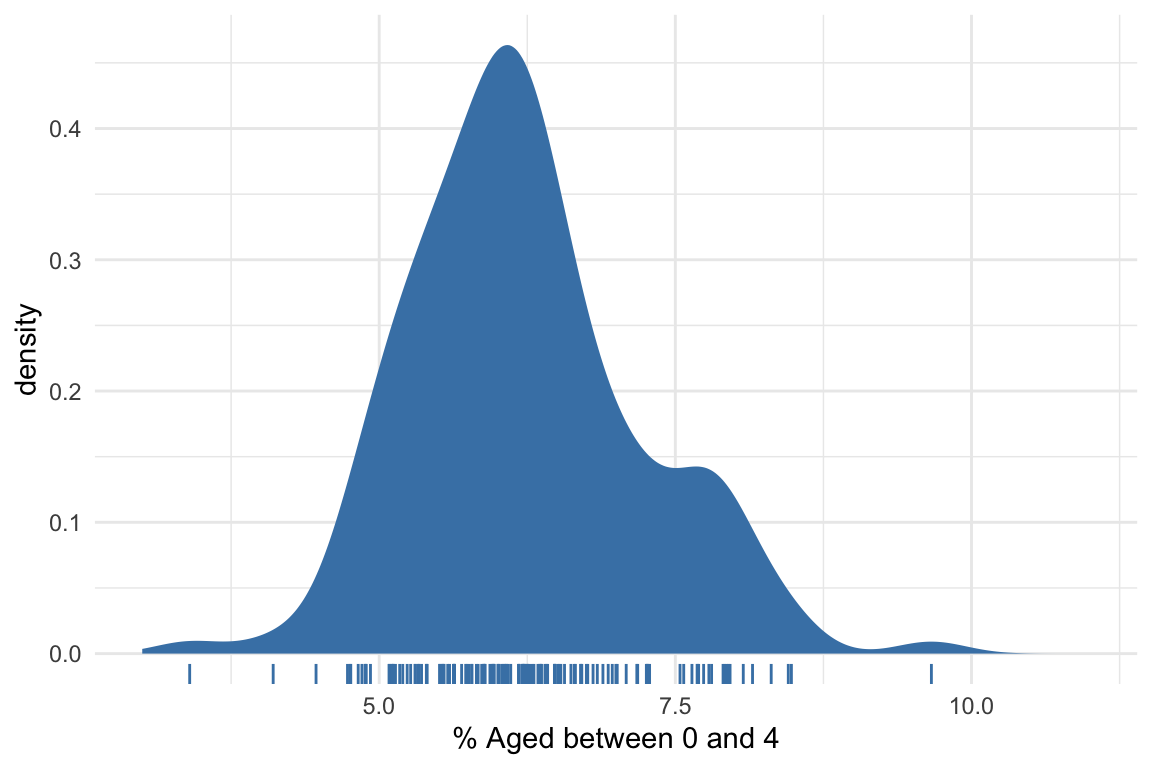

ggplot(data = abs2016,
       aes(x = reorder(State, -Age00_04),
           y = Age00_04,
           colour = State)) +
  geom_boxplot() + 
  theme_minimal() +
  labs(x = "State",
       y = "% Aged between 0 and 4") +
  theme(legend.position = "none") + 
  coord_flip()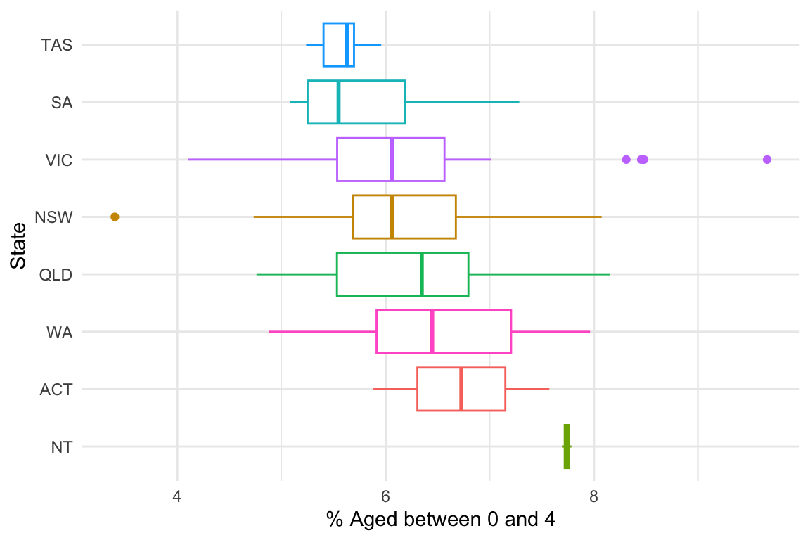

However, there are many age groups. To look at all of them at once, we can gather them into a dataframe ready for plotting using tidyr.

library(tidyr)
library(dplyr)

## 
## Attaching package: 'dplyr'

## The following objects are masked from 'package:stats':
## 
##     filter, lag

## The following objects are masked from 'package:base':
## 
##     intersect, setdiff, setequal, union

abs2016 %>%
  select(starts_with("Age"), 
         DivisionNm) %>%
  gather(key = "Age",
         value = "Percent_in_electorate",
         -DivisionNm) %>% 
  ggplot(data = .,
         aes(x = reorder(Age, - Percent_in_electorate),
             y = Percent_in_electorate,
             colour = Age)) +
  geom_boxplot() + 
  coord_flip() + 
  theme_minimal() + 
  theme(legend.position = "none") +
  labs(x = "Age Groups",
       y = "% in Electorate")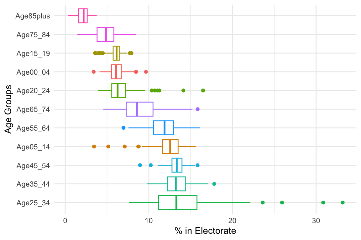

Personal Income

ggplot(data = abs2016,
       aes(x = MedianPersonalIncome)) + 
  geom_density(fill = "salmon",
               bw = "SJ",
               colour = NA) + 
  xlim(250,1100) +
  geom_rug(colour = "salmon") + 
  theme_minimal()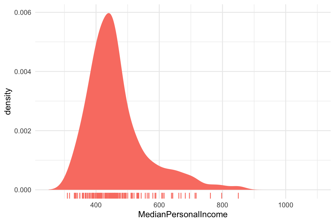

Income by State

ggplot(data = abs2016,
       aes(x = reorder(State, -MedianPersonalIncome),
           y = MedianPersonalIncome,
           colour = State)) + 
  geom_boxplot() + 
  theme_minimal() + 
  theme(legend.position = "none") + 
  labs(x = "State")

If you’re intersted in getting a sense of the distribution of the data, you can add in the points to get a bit more of a sense on the distribution.

ggplot(data = abs2016,
       aes(x = reorder(State, -MedianPersonalIncome),
           y = MedianPersonalIncome,
           colour = State)) + 
  geom_boxplot() + 
  geom_jitter(alpha = 0.35, 
              size = 2,
              width = 0.3) +
  theme_minimal() + 
  theme(legend.position = "none") + 
  labs(x = "State")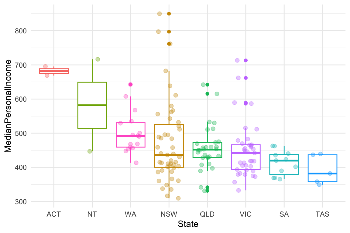

Education

Bachelor and above

ggplot(data = abs2016,
       aes(x = BachelorAbv)) +
  geom_density(fill = "salmon",
               bw = "SJ",
               colour = NA) + 
  geom_rug(colour = "salmon") + 
  theme_minimal() + 
  labs(x = "% of electorate with a Bachelor degree or above") +
  xlim(0, 55)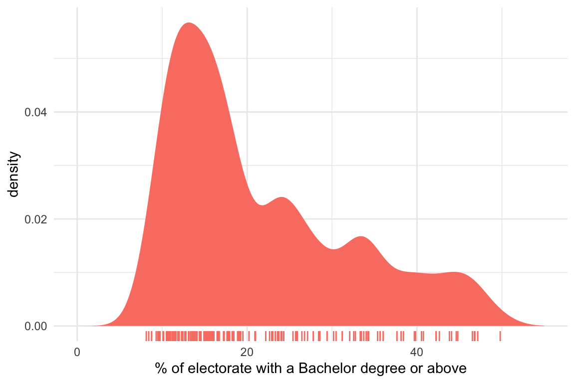

Bachelor by state

ggplot(data = abs2016,
       aes(x = reorder(State, -BachelorAbv),
           y = BachelorAbv,
           colour = State)) +
  geom_boxplot() +
  theme_minimal() +
  labs(x = "State") + 
  theme(legend.position = "none")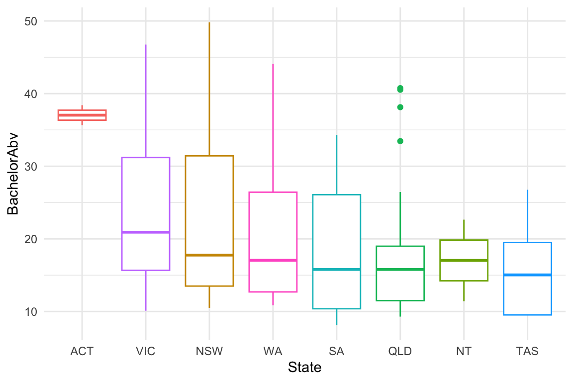

BachelorAbv and income

ggplot(data = abs2016,
       aes(x = BachelorAbv,
           y = MedianPersonalIncome)) + 
  geom_point(colour = "steelblue",
             alpha = 0.75) + 
  theme_minimal()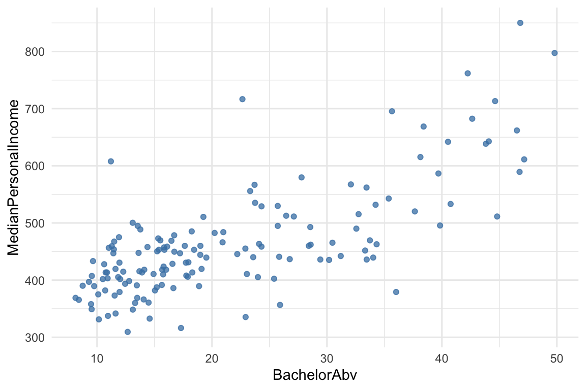

Diploma and Certificate

ggplot(data = abs2016,
       aes(x = reorder(State, -DipCert),
           y = DipCert,
           colour = State)) +
  geom_boxplot() +
  theme_minimal() +
  labs(x = "State") + 
  theme(legend.position = "none")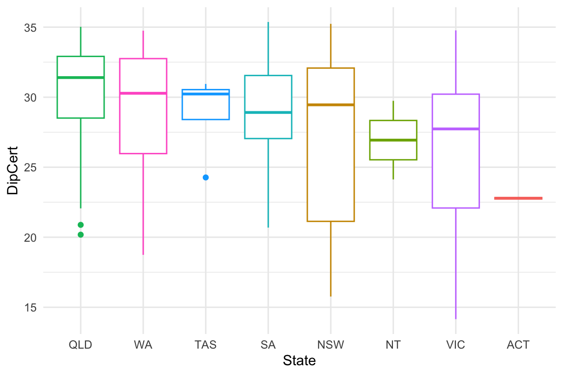

Diploma and Certificate and income

ggplot(data = abs2016,
       aes(x = DipCert,
           y = MedianPersonalIncome)) + 
  geom_point(colour = "steelblue",
             alpha = 0.75) + 
  theme_minimal()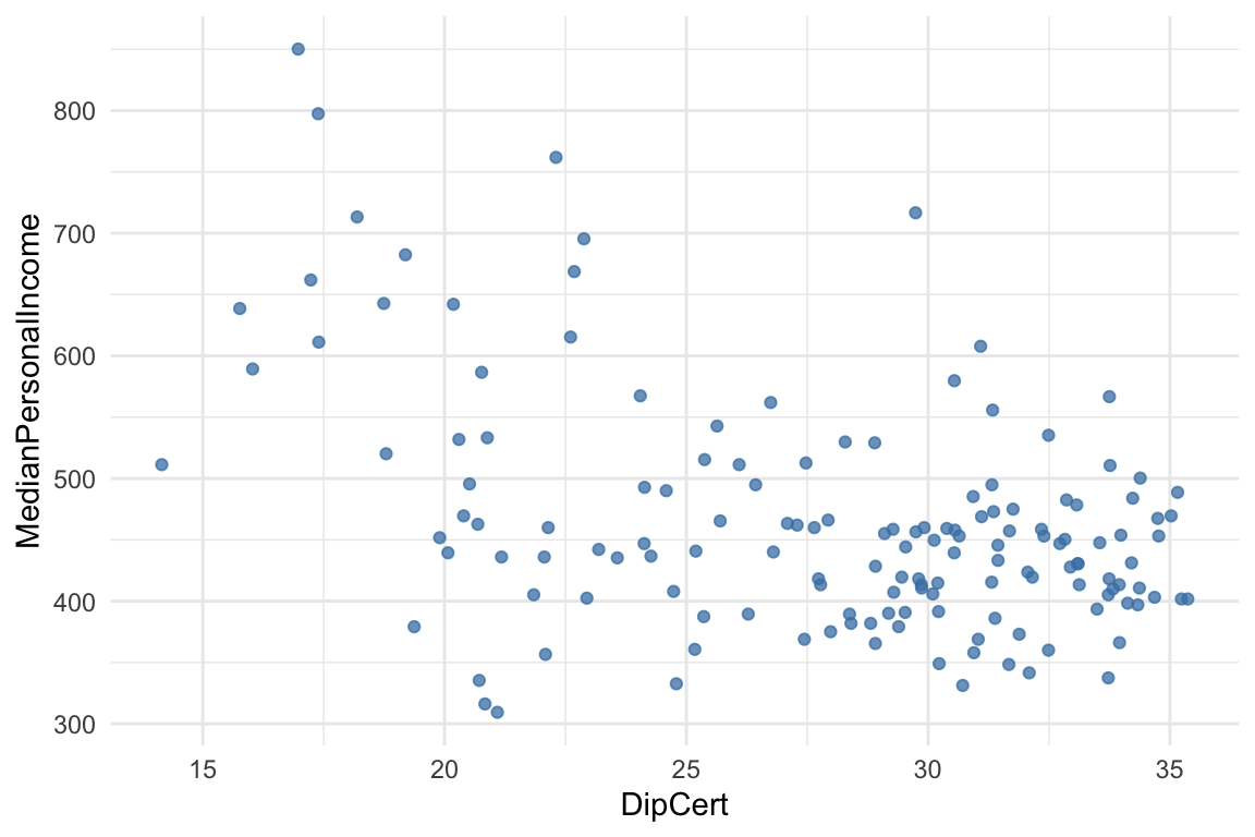

Comparing income across Bachelor (and above) and Diploma/Certificate

abs2016 %>%
  select(DipCert,
         BachelorAbv,
         MedianPersonalIncome) %>% 
  gather(key = "Education",
         value = "Prop_Educated",
         -MedianPersonalIncome) %>%
ggplot(data = ,
       aes(x = Prop_Educated,
           y = MedianPersonalIncome,
           colour = Education)) + 
  geom_point() + 
  geom_smooth() +
  theme_minimal() +
  scale_color_brewer(type = "qual", palette = "Set1")

## `geom_smooth()` using method = 'loess' and formula = 'y ~ x'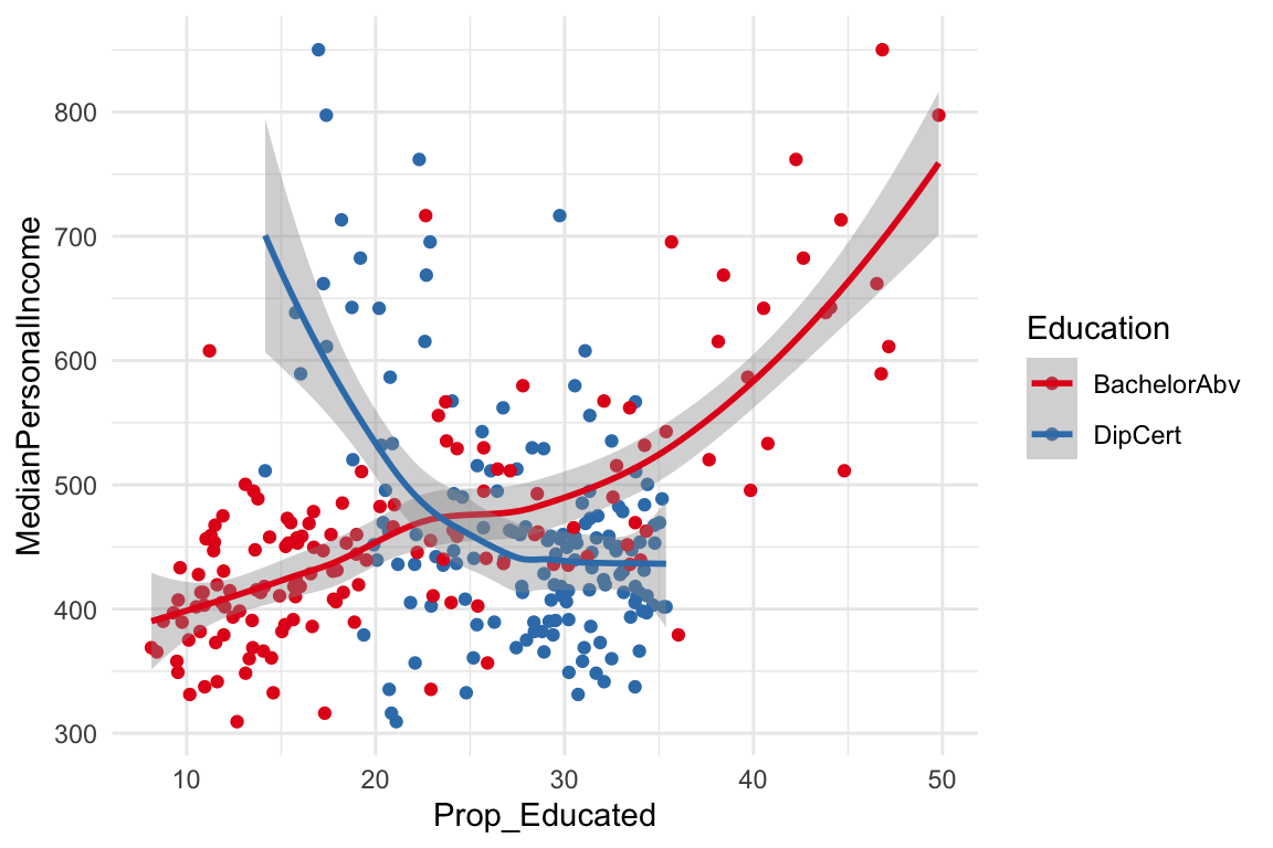

Religion

Let’s look at all of the religions

abs2016 %>%
  select(Christianity,
         Catholic,
         Buddhism,
         Islam,
         Judaism,
         NoReligion) %>%
  gather(key = "ReligionType",
         value = "Percent") %>%
  ggplot(data = .,
         aes(x = reorder(ReligionType, -Percent),
             y = Percent,
             colour = ReligionType)) + 
  geom_boxplot() + 
  theme_minimal() + 
  theme(legend.position = "none") +
  coord_flip() + 
  labs(x = "Religion")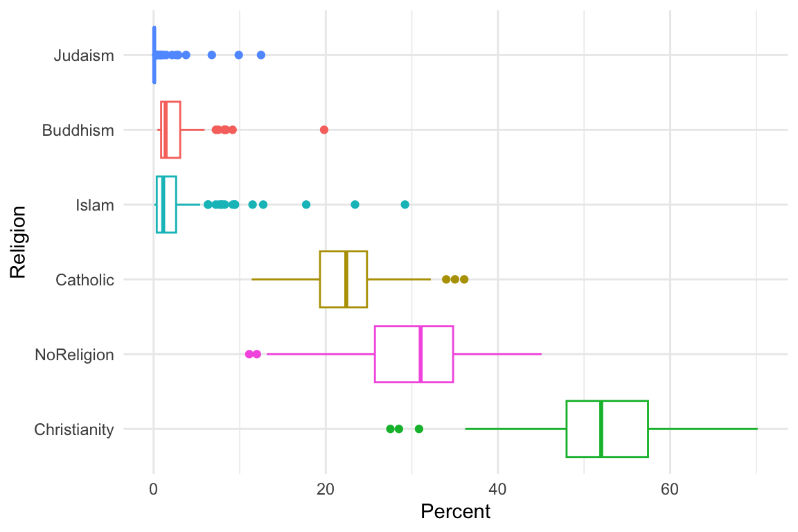

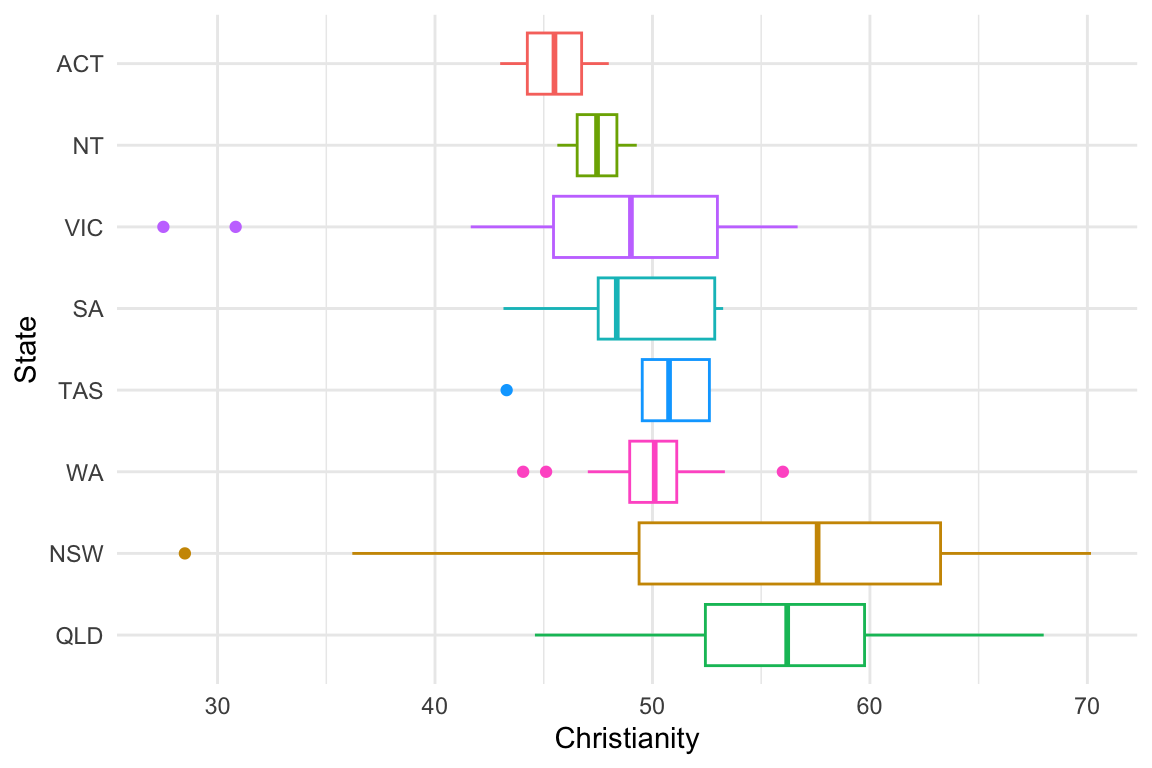
Christianity by State

ggplot(data = abs2016,
       aes(x = reorder(State, -Christianity),
           y = Christianity,
           colour = State)) + 
  geom_boxplot() +
  theme_minimal() +
  theme(legend.position = "none") +
  coord_flip() + 
  labs(x = "State")

Nicholas Tierney, Rob J Hyndman and Jeremy Forbes

2023-04-26